Headline inflation, which refers to the overall change in consumer prices as measured by a broad index, can be heavily influenced by volatile components like energy and food. For example, in a typical year, energy prices might fluctuate by as much as 10% to 30%, while food prices can swing 3% to 8% depending on weather and supply chain disruptions. Central banks often prioritize core inflation—an index that excludes these volatile elements—to better gauge the underlying trend that should inform monetary policy. Investors who react solely to headline inflation risk mispricing assets, potentially causing unnecessary market volatility and missed opportunities.
In addition to supply shocks, cyclical drivers such as a tight labor market can create persistent wage-driven inflation. Wage growth, which often ranges from 2% to 5% annually in developed economies, tends to be more stable than commodity prices, which can reverse course within months. Understanding inflation thus requires careful analysis of labor market indicators (like unemployment rates falling below 4%), productivity growth (which might average 1% to 2% per year), and capacity utilization rates (commonly between 75% and 85% in major economies). These factors collectively shape the pace and persistence of price increases across sectors.
How Inflation Patterns Shift Across Economic Cycles
Inflation does not move uniformly through the business cycle. During economic expansions, wage and input cost pressures build up gradually, often resulting in inflation rising from around 1% to 3% annually until full employment is reached. In contrast, recessions typically bring disinflation or even deflation, with inflation rates dropping to near zero or occasionally turning negative as demand contracts and unemployment rises above 6% or 7%.
Looking at past decades, the 1970s saw annual inflation rates exceeding 10% in some years, driven by oil price shocks and stagnant growth—a phenomenon known as stagflation. By comparison, the post-2008 period featured inflation rates generally between 1% and 2%, even as economies recovered, thanks to productivity gains and subdued wage growth. This contrast highlights that a 3% inflation rate during a robust recovery signals different risks than the same rate during a period of weak growth and high unemployment.
Thus, identical headline inflation figures can mask very different economic realities. Investors must analyze what is driving inflation—whether it is broad-based wage growth, supply chain bottlenecks, or sector-specific shocks—before making asset allocation decisions or adjusting risk premiums.
Statistical Factors That Complicate Inflation Analysis
Several statistical elements contribute to confusion around inflation. Reported inflation figures often reflect conditions from up to six months prior, especially during periods of rapid change. For example, a monthly Consumer Price Index (CPI) release in June may be based on data collected in March or April. Initial estimates are frequently revised by as much as 0.3% to 0.7% after more complete data becomes available, making it risky to base decisions on early releases alone.
Additionally, methodological choices such as hedonic quality adjustments—which estimate how much of a price change is due to improved product features rather than pure inflation—can introduce subtle biases. For instance, if a new smartphone model costs $900 instead of $800 but offers better performance, statisticians might estimate that only $50 of the price increase is true inflation, with the rest attributed to quality improvement. These adjustments, while necessary, can affect long-term trend analysis if not interpreted carefully.
How Asset Prices Reflect Divergent Inflation Expectations
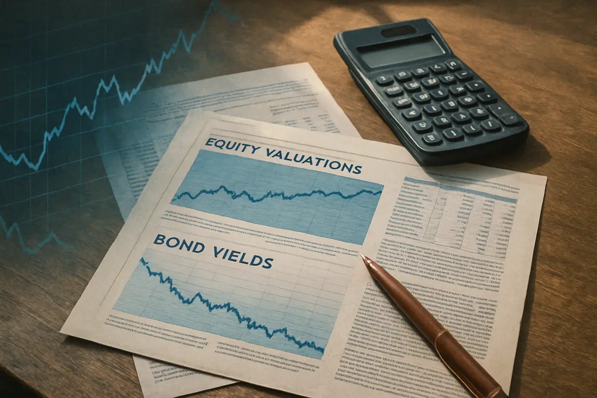
Financial markets do not simply track current inflation; they embed expectations about future price changes, central bank actions, and global events. For example, equities often price in nominal growth and the ability of companies to protect profit margins even as input costs rise. Historically, stock markets have delivered positive real returns during periods of moderate inflation (1% to 3%), but returns can become volatile or negative if inflation exceeds 5% for extended periods.
Bonds, on the other hand, are sensitive to inflation because their fixed interest payments lose purchasing power when prices rise unexpectedly. A 10-year bond yielding 4% annually can see its real return drop to zero if inflation jumps to 4%. Real assets like commodities and real estate often serve as hedges: for instance, gold prices have sometimes surged 20% or more in years of high inflation, while real estate values may appreciate 3% to 6% annually in inflationary environments, though local factors can cause wide variation.
Advantages of Diverse Inflation Indicators
- Offer multiple perspectives on different economic sectors.
- Enable comparison of real-time and lagging trends.
- Support tailored analysis for specific exposures, such as consumer versus producer prices.
Limitations Leading to Misinterpretation
- Complex calculation methods can obscure meaning for non-specialists.
- Volatility in certain categories can distort overall readings temporarily.
- Different reporting schedules create timing mismatches across indicators.
Frequently Misunderstood Aspects of Inflation Measurement
Recognizing common misconceptions is crucial for understanding why market risk premiums often diverge from headline inflation reports. For example, many people believe that the CPI basket is updated annually, when in fact it may only be revised every two to four years. This lag can cause official figures to misrepresent the real-world cost increases faced by households, especially during times of rapid change in consumption habits.
The Trade-Offs in Interpreting Inflation Data
Every inflation measure balances the need for timely data with the accuracy provided by rigorous statistical methods. This trade-off means that initial reports may be incomplete, and subsequent revisions can alter the perceived inflation trend by up to 0.5 percentage points. For investors and policymakers, this creates a challenge: relying on early data can lead to premature decisions, while waiting for more accurate figures may mean missing critical inflection points in the economy.
No single inflation statistic captures the full range of price changes across different sectors, regions, or consumer groups. For example, while the national inflation rate may average 2% to 3%, urban households could experience increases of 4% or more in housing costs, while rural residents might see stable or declining rents. This diversity requires a holistic approach to analysis, combining headline numbers with sector-specific and demographic information to avoid over- or underestimating inflation risk.
How Consumer Behavior Shapes Real Inflation Impact
Consumer reactions to inflation are neither uniform nor predictable. When prices rise rapidly—say, food costs jump 8% year-over-year—consumers may accelerate purchases of nonperishable goods, temporarily boosting demand and further driving up prices. Conversely, if inflation expectations drop, discretionary spending may slow, dampening economic growth. This behavioral feedback loop complicates both the measurement and forecasting of inflation, as it influences the velocity of money—the rate at which money circulates through the economy—which itself can vary from 1.2 to 2.0 times GDP in major economies.
Substitution effects also matter. If beef prices rise 15% in a year, many consumers switch to less expensive proteins, such as chicken or plant-based options, muting the impact of price increases on their overall food budget. Official inflation measures attempt to reflect these changes by periodically adjusting the "basket" of goods and services, but these updates may lag behind actual shifts in consumer preferences, especially during volatile periods.
Inflation is also experienced differently across demographic and geographic groups. Lower-income households, which may spend 30% to 40% of their budget on food and energy, feel the brunt of price spikes in these categories more acutely than higher-income households, who might spend only 10% to 15% on such essentials. Similarly, housing costs can rise by 5% to 10% annually in high-demand urban centers, while remaining flat or even declining in smaller towns. Policymakers who rely solely on aggregate inflation figures risk missing the unique pressures faced by specific populations.
Inflation also affects investment portfolios unevenly. Equities may benefit from nominal revenue growth during moderate inflation, but fixed-income securities—like bonds with a 3% coupon—lose real value if inflation rises to 4% or higher. Real estate can serve as a partial hedge, but local market trends may override national inflation rates. To accurately assess portfolio risk, investors need to consider sector-specific inflation data, forward-looking indicators such as breakeven inflation rates (the difference between yields on standard Treasury bonds and Treasury Inflation-Protected Securities, or TIPS), and global economic conditions.
Data lag is another challenge. Inflation statistics are typically published monthly but reflect transactions from several weeks prior. For example, if a supply chain disruption causes a 20% spike in commodity prices in February, the official inflation report released in March may not fully capture the impact until April or May. Real-time data sources—such as credit card transaction records or online price tracking—can help, but integrating these into official statistics remains complex.
Core inflation, which excludes food and energy, is designed to reveal persistent trends by removing volatile categories. However, since food and energy often make up 20% to 25% of household spending and can see price swings of 10% or more in a single year, excluding them can understate the immediate financial pressure felt by consumers. For analysts, comparing headline and core inflation rates—such as a 4% headline versus a 2.5% core rate—can provide insight into whether price increases are likely to persist or fade.
A Step-by-Step Example: Calculating Real Bond Returns in an Inflationary Year
Suppose you invest $10,000 in a 5-year bond with a 4% annual coupon. Over one year, you receive $400 in interest. If inflation for that year is 3%, your real return is calculated as follows:
- Nominal return: $400 (4% of $10,000)
- Inflation adjustment: $10,000 x 3% = $300
- Real return: $400 - $300 = $100, or 1% of your principal
This calculation illustrates that even when nominal interest rates appear attractive, real (inflation-adjusted) returns can be much lower—sometimes less than half the nominal rate—if inflation is higher than expected.
Practical Implications for Financial Decision-Making
Given the complexities of inflation measurement and interpretation, both individuals and professionals should be cautious about relying solely on headline figures. For example, a retiree whose expenses are indexed to the CPI might face unexpected shortfalls if their personal inflation rate—driven by healthcare or housing—runs 2% to 3% above the national average. Similarly, businesses must anticipate not only rising input costs but also potential shifts in consumer demand as inflation expectations change.
Portfolio diversification is essential. Allocating assets across categories with different inflation sensitivities—such as equities, real estate, commodities, and inflation-indexed securities like TIPS—can help manage risk. However, these strategies have trade-offs: commodities and real estate can be illiquid or volatile, and TIPS may underperform during periods of low or negative inflation.
Why Measuring Inflation Is Inherently Complex
Inflation is not a single, universal rate but a composite of price movements across dozens of categories, from housing and transportation to healthcare and technology. For example, technology prices may decline 3% to 7% per year due to innovation, while healthcare costs can climb 4% to 6% annually. As a result, the official inflation rate—often reported as a single figure between 2% and 4%—can conceal substantial variation in the cost of living across households.
Measures like the Consumer Price Index (CPI) rely on a representative basket of goods and services, which may be updated only every 2 to 4 years. This lag means that rapid changes in consumer habits or the introduction of new products can be missed, causing the official inflation rate to overstate or understate actual cost increases. For example, if a new technology reduces the cost of communication by $20 per month, but the CPI basket is not updated to reflect this, the true improvement in living standards may go unnoticed.
Furthermore, the publication lag—often three months or more—means that inflation data can be out of sync with current conditions. During periods of rapid change, such as a sudden spike in oil prices, this delay can result in decisions being made on outdated information, complicating both investment and policy responses.
Behavioral Biases That Skew Inflation Perceptions
Behavioral factors play a major role in how people perceive inflation. The availability heuristic leads individuals to focus on recent or highly visible price changes—such as a 25% jump in gasoline prices—while overlooking stable or declining prices elsewhere. This can cause perceived inflation to exceed the actual average, particularly during periods of high media coverage.
Anchoring bias causes people to compare current prices to outdated reference points, such as remembering when a loaf of bread cost $1.50 instead of the current $2.50. This can distort perceptions, especially if product sizes or quality have changed. Loss aversion further amplifies the emotional impact of price increases, making a 5% rise in rent feel more significant than a 5% drop in the price of electronics.
Social and media influences can reinforce these biases, particularly when alarming headlines or group discussions focus on extreme examples. Combined with limited financial literacy—studies suggest that only 30% to 40% of adults can accurately define inflation—these factors create widespread misunderstanding of how inflation affects personal finances.
Practical Implications for Investors and Consumers
Misjudging inflation can have significant financial consequences. Investors who overestimate future inflation may shift too heavily into cash or short-term bonds, which often yield less than 2% after inflation, missing out on higher long-term returns from equities or real assets. Conversely, underestimating inflation can erode purchasing power, especially for retirees or others on fixed incomes.
For consumers, misunderstanding inflation can lead to poor budgeting and savings decisions. If a household expects inflation to be 2% but actual costs rise 4%, they may find themselves short on savings within a few years. Adjusting savings goals and spending plans to account for realistic inflation ranges—typically 2% to 4% annually—can help preserve financial stability over time.
Case Study: The Impact of Inflation Misjudgment on Retirement Planning
Consider the case of a retiree who plans for a 2% annual inflation rate. If healthcare and property taxes—representing 30% of their expenses—rise by 5% per year, while the rest of their budget increases by 2%, their overall cost of living could rise by 3% to 3.5% annually. Over five years, a $40,000 annual budget would need to grow to about $46,400 to keep pace—a $6,400 difference that could deplete savings faster than planned. This example underscores the importance of tracking personal inflation rates and periodically revisiting assumptions when making long-term financial plans.